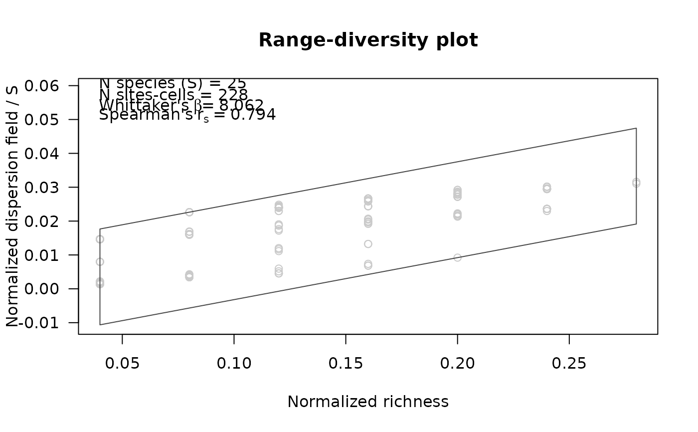
Representations of diversity and dispersion indices

Graphic representations of results from prepare_PAM_CS. Plots present the new range-diversity diagram and geographic views of results. Geographic representations are only possible when significant analyses were performed.

Usage

plot_PAM_CS(PAM_CS, add_significant = FALSE,
            add_random_values = FALSE, col_all = "#CACACA",
            col_significant_low = "#6D6D6D",
            col_significant_high = "#000000",
            col_random_values = "#D2D2D2", pch_all = 1,
            pch_significant_low = 16, pch_significant_high = 16,
            pch_random_values = 1, main = NULL,
            xlab = NULL, ylab = NULL, xlim = NULL, ylim = NULL,
            ylim_expansion = 0.25, las = 1, add_legend = TRUE)

plot_PAM_CS_geo(PAM_CS, xy_coordinates = NULL, col_all = "#CACACA",
                col_significant_low = "#6D6D6D",
                col_significant_high = "#000000", border = NULL,
                pch_all = 16, pch_significant_low = 16,
                pch_significant_high = 16, xlim = NULL,
                ylim = NULL, mar = NULL)

Arguments

PAM_CS: object of class PAM_CS or a base_PAM object containing a PAM_CS object as part of PAM_indices. These objects can be obtained using the function prepare_PAM_CS.
add_significant: (logical) whether to add statistically significant values using a different symbol. Default = FALSE. If TRUE and values indicating significance are not in PAM_CS, a message will be printed.
add_random_values: (logical) whether to add values resulted from the randomization process done when preparing PAM_CS. Default = FALSE. Valid only if add_significant = TRUE, and randomized values are present in PAM_CS.
col_all: color code or name for all values or those that are not statistically significant. Default = "#CACACA".
col_significant_low: color code or name for significant values below confidence limits of random expectations. Default = "#000000".
col_significant_high: color code or name for significant values above confidence limits of random expectations. Default = "#000000".
col_random_values: color code or name for randomized values. Default = "D2D2D2".
pch_all: point symbol to be used for all values. Defaults = 1 or 16.
pch_significant_low: point symbol to be used for significant values below confidence limits of random expectations. Default = 16.
pch_significant_high: point symbol to be used for significant values above confidence limits of random expectations. Default = 16.
pch_random_values: point symbol to be used for randomized values. Default = 1.
main: main title for the plot. Default = NULL.
xlab: label for the x-axis. Default = NULL.
ylab: label for the y-axis. Default = NULL.
xlim: x limits of the plot (x1, x2). For plot_PAM_CS, the default, NULL, uses the range of normalized richness.
ylim: y limits of the plot. For plot_PAM_CS, the default, NULL, uses the range of the normalized values of the dispersion field. The second limit is increased by adding the result of multiplying it by ylim_expansion, if add_legend = TRUE.
ylim_expansion: value used or expanding the ylim. Default = 0.25.
las: the style of axis labels; default = 1. See par.
add_legend: (logical) whether to add a legend describing information relevant for interpreting the diagram. Default = TRUE.
xy_coordinates: Only required if PAM_CS is of class PAM_CS. A matrix or data.frame containing the columns longitude and latitude (in that order) corresponding to the points in PAM_CS$S_significance_id. Default = NULL
border: color for cell borders of the PAM grid. The default, NULL, does not plot any border.
mar: (numeric) vector of length 4 to set the margins of the plot in geography. The default, NULL, is (3.1, 3.1, 2.1, 2.1).

Value

For plot_PAM_CS:

A range-diversity plot with values of normalized richness in the x-axis, and normalized values of the dispersion field index divided by number of species in the y-axis.

For plot_PAM_CS_geo:

A geographic view of the PAM representing the areas or points identified as non statistically significant, significant above random expectations, and significant below random expectations.

Examples

# Data
b_pam <- read_PAM(system.file("extdata/b_pam.rds",
                              package = "biosurvey"))

# Preparing data for CS diagram
pcs <- prepare_PAM_CS(PAM = b_pam)

# Plot
plot_PAM_CS(pcs)